New year is coming soon, so many companies are planning their budgets for the next year these days. Cost estimations are often require DAU forecast. In this article I’ll show you how you can get this prediction using the Duolingo’s growth model and share a DAU & MAU “calculator” designed as a Google Spreadsheet calculator.
2. Methodology
A quick recap on how the Duolingo’s growth model works. At day \(d\) (\(d=1,2,\ldots,\)) of a user’s lifetime the user can be in one of the following 7 (mutually-exclusive) states:
state
d = 1
active today
active in [d-6, d-1]
active in [d-29, d-7]
active before d-30
new
✅
?
NA
NA
NA
current
❌
✅
✅
❓
❓
reactivated
❌
✅
❌
✅
?
resurrected
❌
✅
❌
❌
✅
at_risk_wau
❌
❌
✅
?
?
at_risk_mau
❌
❌
❌
✅
?
dormant
❌
❌
❌
❌
✅
Having these states defined (as set \(S\)), we can consider a user’s lifetime trajectory as a Markov chain. Let \(M\) be a transition matrix associated with this Markov chain: \(m_{i, j} = P(s_j | s_i)\) are the probabilities that a user moves to state \(s_j\) right after being at state \(s_i\), \(s_i, s_j \in S\). The matrix values are easily fetched from the historical data.
If we assume that the user behavior is stationary, the matrix \(M\) fully describes states of the all users in the future. Suppose that vector \(u_0\) of length 7 contains the counts of users being in certain states at some calendar day denoted as 0. Thus, according to the Markov model, in the next day \(u_1\) we expect to have the following amount of users:
Applying this formula recursevely, we derive the amount of the users at any arbitrary day \(t > 0\) in the future. The only thing we need to provide despite of the initial distribution \(u_0\) is to the amount of new users that would appear in the product each day in the future. We’ll get it by using historical data on new users appeared in the past and appyling the prophet library.
Now, having \(u_t\) calculated, we can calculate DAU values at day t: \[DAU_t = \#New_t + \#Current_t + \#Reactivated_t +\#Resurrected_t.\]
Additionally, we can easily calculate WAU and MAU metrics: \[WAU_t = DAU_t +\#AtRiskWau_t,\]\[MAU_t = DAU_t +\#AtRiskWau_t + \#AtRiskMau_t.\]
Finally, the algorithm looks like this:
For each prediction day \(t=1, ..., T\) calculate the expected amount of new users \(\#New_1, \ldots, \#New_T\).
For each lifetime day of each user define on of the 7 states.
Calculate the transition matrix \(M\).
Calculate initial counts \(u_0\) corresponding to \(t=0\) day.
Calculate recursively \(u_{t+1} = M^T u_t\).
Calculate DAU, WAU, MAU for each prediction day \(t=1, ..., T\).
3. Implementation
3.1 Dataset
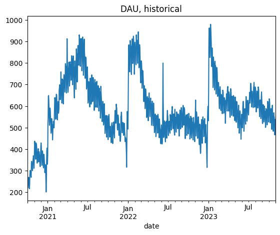
We use a simulated dataset based on historical data of a SAAS app. The data is stored in the dau_data.csv.gz file and contains three columns: user_id, date, and registration_date. Each record indicates a day when a user was active.
The data includes activity indicators for all users from 2020-11-01 to 2023-10-31. An additional month, October 2020, is included to calculate user states correctly (at_risk_mau and dormant states require data from one month prior).
Suppose that today is 2022-10-31 and we want to predict the DAU metric for the next 2023 year. We define a couple of constants PREDICTION_START and PREDICTION_END which define the prediction period.
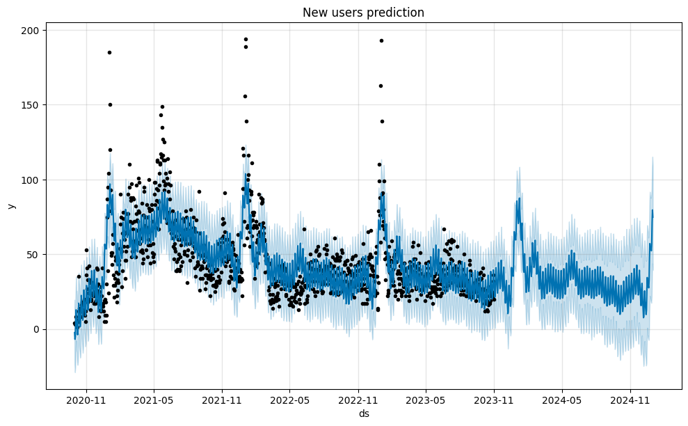
Let’s start from the new users prediction. We use the prophet library as one of the easiest ways to predict time-series data. The new_users Series contains such data. We extract it from the original df dataset selecting the rows where the registration date is equal to the date.
prophet requires a time-series as a DataFrame containing two columns ds and y, so we reformat the new_users Series to the new_users_prophet DataFrame. Another thing we need to prepare is to create the future variable containing certain days for prediction: from PREDICTION_START to PREDICTION_END. The plot illustrates predictions for both past and future dates.
/Users/v.kukushkin/Documents/private/wowone.github.io/.venv/lib/python3.12/site-packages/tqdm/auto.py:21: TqdmWarning: IProgress not found. Please update jupyter and ipywidgets. See https://ipywidgets.readthedocs.io/en/stable/user_install.html
  from .autonotebook import tqdm as notebook_tqdm
In practice, the most calculations are reasonable to execute as SQL queries to a database where the data is stored. Hereafter, we will simulate such quering with the duckdb library.
We want to assign one of the 7 states to each day of a user’s lifetime within the app. According to the definition, for each day, we need to consider at least the past 30 days. This is where SQL window functions come in. However, since the df data contains only records of active days, we need to explicitly extend it to include the days when a user was not active. In other words, instead of this list of records:
user_id    date          registration_date
1234567    2023-01-01    2023-01-01
1234567    2023-01-03    2023-01-01
For readability purposes we split the following SQL query into multiple subqueries.
full_range: Create a full sequence of dates for each user.
dau_full: Get the full list of both active and inactive records.
states: Assign one of the 7 states for each day of a user’s lifetime.
Toggle the code
import duckdbDATASET_START ='2020-11-01'DATASET_END ='2023-10-31'OBSERVATION_START ='2020-10-01'query =f"""WITHfull_range AS ( SELECT user_id, UNNEST(generate_series(greatest(registration_date, '{OBSERVATION_START}'), date '{DATASET_END}', INTERVAL 1 DAY))::date AS date FROM ( SELECT DISTINCT user_id, registration_date FROM df )),dau_full AS ( SELECT fr.user_id, fr.date, df.date IS NOT NULL AS is_active, registration_date FROM full_range AS fr LEFT JOIN df USING(user_id, date)),states AS ( SELECT user_id, date, is_active, first_value(registration_date IGNORE NULLS) OVER (PARTITION BY user_id ORDER BY date) AS registration_date, SUM(is_active::int) OVER (PARTITION BY user_id ORDER BY date ROWS BETWEEN 6 PRECEDING and 1 PRECEDING) AS active_days_back_6d, SUM(is_active::int) OVER (PARTITION BY user_id ORDER BY date ROWS BETWEEN 29 PRECEDING and 1 PRECEDING) AS active_days_back_29d, CASE WHEN date = registration_date THEN 'new' WHEN is_active = TRUE AND active_days_back_6d BETWEEN 1 and 6 THEN 'current' WHEN is_active = TRUE AND active_days_back_6d = 0 AND IFNULL(active_days_back_29d, 0) > 0 THEN 'reactivated' WHEN is_active = TRUE AND active_days_back_6d = 0 AND IFNULL(active_days_back_29d, 0) = 0 THEN 'resurrected' WHEN is_active = FALSE AND active_days_back_6d > 0 THEN 'at_risk_wau' WHEN is_active = FALSE AND active_days_back_6d = 0 AND ifnull(active_days_back_29d, 0) > 0 THEN 'at_risk_mau' ELSE 'dormant' END AS state FROM dau_full)SELECT user_id, date, state FROM statesWHERE date BETWEEN '{DATASET_START}' AND '{DATASET_END}'ORDER BY user_id, date"""states = duckdb.sql(query).df()
The query results are kept in the states DataFrame:
states.head()
user_id
date
state
0
00002b68-adba-5a55-92d7-8ea8934c6db3
2023-06-23
new
1
00002b68-adba-5a55-92d7-8ea8934c6db3
2023-06-24
current
2
00002b68-adba-5a55-92d7-8ea8934c6db3
2023-06-25
current
3
00002b68-adba-5a55-92d7-8ea8934c6db3
2023-06-26
current
4
00002b68-adba-5a55-92d7-8ea8934c6db3
2023-06-27
current
3.4 Calculating the transition matrix
Having obtained these states, we can calculate state transition frequencies. In the real world, due to the large amount of data, it would be more effective to use a SQL query rather than a Python script. We calculate these frequencies day-wise since we’re going to study how the prediction depends on the period in which transitions are considered further.
Toggle the code
query =f"""SELECT date, state_from, state_to, COUNT(*) AS cnt,FROM ( SELECT date, state AS state_to, lag(state) OVER (PARTITION BY user_id ORDER BY date) AS state_from FROM states)WHERE state_from IS NOT NULLGROUP BY date, state_from, state_toORDER BY date, state_from, state_to;"""transitions = duckdb.sql(query).df()
The result is stored in the transitions DataFrame.
transitions.head()
date
state_from
state_to
cnt
0
2020-11-02
at_risk_mau
at_risk_mau
273
1
2020-11-02
at_risk_mau
dormant
4
2
2020-11-02
at_risk_mau
reactivated
14
3
2020-11-02
at_risk_wau
at_risk_mau
18
4
2020-11-02
at_risk_wau
at_risk_wau
138
Now, we can calculate the transition matrix \(M\). We define the get_transition_matrix function, which accepts the transitions DataFrame and a pair of dates that bounds the transitions to be considered.
As a baseline, let’s calculate the transition matrix for the whole year from 2021-11-01 to 2022-10-31.
M = get_transition_matrix(transitions, '2022-11-01', '2023-10-31')M
state_to
new
current
reactivated
resurrected
at_risk_wau
at_risk_mau
dormant
state_from
new
0.0
0.515934
0.000000
0.000000
0.484066
0.000000
0.000000
current
0.0
0.851325
0.000000
0.000000
0.148675
0.000000
0.000000
reactivated
0.0
0.365867
0.000000
0.000000
0.634133
0.000000
0.000000
resurrected
0.0
0.316474
0.000000
0.000000
0.683526
0.000000
0.000000
at_risk_wau
0.0
0.098246
0.004472
0.000000
0.766263
0.131020
0.000000
at_risk_mau
0.0
0.000000
0.009598
0.000173
0.000000
0.950109
0.040120
dormant
0.0
0.000000
0.000000
0.000387
0.000000
0.000000
0.999613
3.5 Getting the initial state counts
An initial state is easily retrieved from the states DataFrame by the get_state0 function and the corresponding SQL query. We assign the result to the state0 variable.
Toggle the code
def get_state0(date): query =f""" SELECT state, count(*) AS cnt FROM states WHERE date = '{date}' GROUP BY state """ state0 = duckdb.sql(query).df() state0 = state0.set_index('state').reindex(states_order)['cnt']return state0
state0 = get_state0(DATASET_END)state0
state
new               20
current          475
reactivated       15
resurrected       19
at_risk_wau      404
at_risk_mau     1024
dormant        49523
Name: cnt, dtype: int64
3.6 Predicting DAU
The predict_dau function below accepts all the previous variables required for the DAU prediction and makes this prediction for a date range defined by the start_date and end_date arguments.
Toggle the code
def predict_dau(M, state0, start_date, end_date, new_users):""" Predicts DAU over a given date range. Parameters ---------- M : pandas.DataFrame Transition matrix representing user state changes. state0 : pandas.Series counts of initial state of users. start_date : str Start date of the prediction period in 'YYYY-MM-DD' format. end_date : str End date of the prediction period in 'YYYY-MM-DD' format. new_users : int or pandas.Series The expected amount of new users for each day between `start_date` and `end_date`. If a Series, it should have dates as the index. If an int, the same number is used for each day. Returns ------- pandas.DataFrame DataFrame containing the predicted DAU, WAU, and MAU for each day in the date range, with columns for different user states and tot. """ dates = pd.date_range(start_date, end_date) dates.name ='date' dau_pred = [] new_dau = state0.copy()for date in dates: new_dau = (M.transpose() @ new_dau).astype(int)ifisinstance(new_users, int): new_users_today = new_userselse: new_users_today = new_users.astype(int).loc[date] new_dau.loc['new'] = new_users_today dau_pred.append(new_dau.tolist()) dau_pred = pd.DataFrame(dau_pred, index=dates, columns=states_order) dau_pred['dau'] = dau_pred['new'] + dau_pred['current'] + dau_pred['reactivated'] + dau_pred['resurrected'] dau_pred['wau'] = dau_pred['dau'] + dau_pred['at_risk_wau'] dau_pred['mau'] = dau_pred['dau'] + dau_pred['at_risk_wau'] + dau_pred['at_risk_mau']return dau_pred
Besides the expected dau, wau, and mau columns, the output contains the number of users in each state for each prediction date.
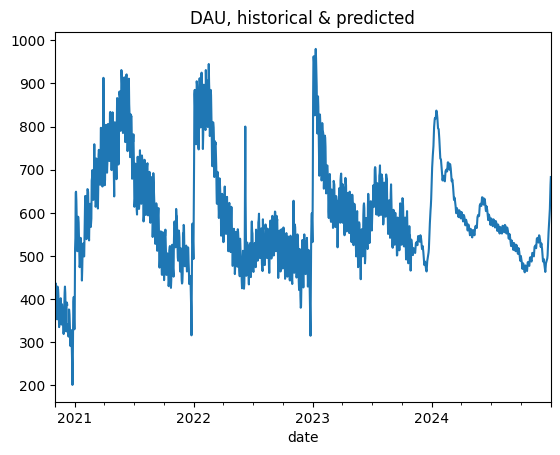
Finally, we calculate the ground-truth values of DAU, WAU, and MAU (along with the corresponding state decomposition), keep them in the dau_true DataFrame, and plot the predicted and true values altogether.
First of all, let’s check whether we really need to build a complex model to predict DAU. Wouldn’t it be better to predict DAU as a general time-series using the mentioned prophet library? The function predict_dau_simple implements this. We try to use some tweaks available in the library in order to make the prediction more accurate:
we use logistic model instead of linear in order to avoid negative values;
we add explicitly monthly and yearly seasonality;
we remove the outliers.
we set explicitly define peak values for January and February as “holidays”.
The fact that the code turns out to be quite sophisticated indicates that one can’t simply apply prophet to the DAU time-series.
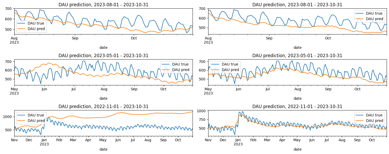
The MAPE error turns out to be high: 18% - 35%. The fact that the shortest horizont has the highest error means that the model is tuned for the long-term predictions. This is another inconvenience of such an approach: we have to tune the model for each prediction horizont. So this is our baseline. In the next section we’ll compare it with the more advanced models.
4.2 General evaluation
In this section we evaluate the model implemented in the section 3. So far we set the transition period as 1 year before the prediction start. We’ll study how the prediction depends on the transition period in the next section. As for the new users, we run the model using two options: the real values and the predicted ones. Similarly, we fix the same 3 prediction horizonts and test the model on them.
The make_predicion function below implements the described opttions. It accepts prediction_start, prediction_end arguments defining the prediction period for a given horizont, new_users_mode which can be either true or predict, and transition_period.
In general, the model demonstrates much better results than the baseline. Indeed, the baseline is based on the historical DAU data only, while the model uses the user states information.
However, for the 1-year horizont and new_users_mode='predict' the MAPE error is huge: 65%. This is 3 times higher than the corresponding baseline error (21%). On the other hand, new_users_mode='true' option gives a much better result: 8%. It means that the new users prediction has a huge impact on the model, especially for long-term predictions. For the shorter periods the difference is less dramatic. The major difference for such a difference is that 1-year period includes Christmas with its extreme values. As a result, i) it’s hard to predict such high new user values, ii) the period heavily impacts user behavior, the transition matrix and, consequently, DAU values. Hence, we strongly recommend to implement the new user prediction carefully. The baseline model was specially tuned for this Christmas period, so it’s not surprising that it outperforms the Markov model.
When the new users prediction is accurate, the model captures trends well. It means that using last 365 days for the transition matrix calculation is a reasonable choice.
Interestingly, the true new users data provides worse results for the 3-months prediction. This is nothing but a coincidence. The wrong new users prediction in October 2023 reversed the predicted DAU trend and made MAPE a bit lower.
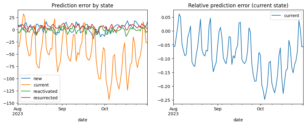
Now, let’s decompose the prediction error and see which states contribure the most. Since we already know that the new users prediction has a huge impact on the model, we focus on a shorter prediction period in order to study the other factors.
From the left chart we notice that the error is basically contributed by the current state. It’s not surprising since this state contributes to DAU the most. The error for the new, reactivated, and resurrected states is quite low. Another interesting thing is that this error is mostly negative. Perhaps it mean that the new users who appeared in the prediction period are more engaged that the users from the past.
As for the relative error on the right chart, it makes sense to analyze it for the current state only. This is because the daily amount of the reactivated and resurrected states are low so the relative error is high and noisy. The relative error for the current state varies between -20% and 5% which is quite high. And since the current state amount is mostly regulated by the current -> current conversion rate (it’s roughly 0.8), this error is explained by the transition matrix inaccuracy.
4.3 Transitions period impact
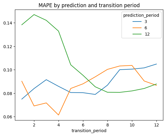
In the previous section we kept the transitions period fixed – 1 year before a prediction start. Now we’re going to study how long this period should be to get more accurate prediction. We consider the same prediction horizonts of 3, 6, and 12 months. In order to mitigate the noise from the new users prediction, we use the real values of the new users amount.
It turns out that the optimal transitions period depends on the prediction horizont. Shorter horizonts require shorter transitions periods: the minimal MAPE error is achieved at 1, 4, and 8 transition periods for the 3, 6, and 12 months correspondingly. It seems this is because the longer horizonts contain some seasonal effects that could be captured only by the longer transitions periods.
4.4 Obsolence and seasonality
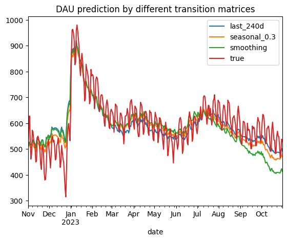
Nevertheless, fixing a single transition matrix for predicting the whole year ahead doesn’t seem to be a good idea: such a model would be too rigid. Usually, the user behavior varies depending on a season. For example, users who appear after Christmas might have some shifts in behavior. Another typical situation is when users change their behavior in summer. In this section, we’ll try to take into account these seasonal effects.
So we want to predict DAU for the 1 year ahead starting from November 2022. Instead of using a single transition matrix \(M_{base}\) which is calculated for the last 8 months before the prediction start (as an optimal transitions period derived from the previous section, labeled as last_240d option), we’ll consider a mixture of this matrix and a seasonal one \(M_{seasonal}\). The latter is calculated on monthly basis lagging 1 year behind. For example, to predict DAU for November 2022 we define \(M_{seasonal}\) as the transition matrix for November 2021. Then we shift the prediction horizon to December 2022 and calculate \(M_{seasonal}\) for December 2021, etc.
In order to mix \(M_{base}\) and \(M_{seasonal}\) we define the following two options.
seasonal_0.3: \(M = 0.3 \cdot M_{seasonal} + 0.7 \cdot M_{base}\). 0.3 weight was chosen as a local minimum after some experiments.
smoothing: \(M = \frac{i}{N - 1} M_{seasonal} + (1 - \frac{i}{N - 1}) M_{base}\) where \(N\) is the number of months within the predicting period, \(i = 0, \ldots, N - 1\) – the month index. The idea of this configuration is to gradually switch from the most recent transition matrix \(M_{base}\) to seasonal ones as the prediction month moves forward from the prediction start.
Toggle the code
result = pd.DataFrame()for transition_period in ['last_240d', 'seasonal_0.3', 'smoothing']: result[transition_period] = make_prediction('2022-11-01', '2023-10-31', 'true', transition_period)['dau']result['true'] = dau_true['dau']result['true'] = result['true'].astype(int)result.plot(title='DAU prediction by different transition matrices');
Toggle the code
mape = pd.DataFrame()for col in result.columns:if col !='true': mape.loc[col, 'mape'] = mean_absolute_percentage_error(result['true'], result[col])mape
mape
last_240d
0.080804
seasonal_0.3
0.077545
smoothing
0.097802
According to the MAPE errors, seasonal_0.3 configuration provides the best results. Interestingly, smoothing approach has appeared to be even worse than the last_240d. From the diagram above we see that all three models start to underestimate the DAU values from July 2023, especially the smoothing model. It seems that the new users who started appearing from July 2023 are more engaged than the users from 2022. Probably, the app was improved sufficiently or the marketing team did a great job. As a result, the smoothing model that much relies on the outdated transitions data from July 2022 - October 2022 fails more than the other models.
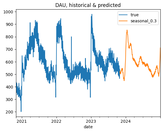
4.5 Final solution
To sum things up, let’s make a final prediction for the 2024 year. We use the seasonal_0.3 configuration and the predicted values for new users.
In the section 4 we studied the model performance from the prediction accuracy perspective. Now let’s discuss the model from the practical point of view. We compare it with the baseline model (see the section 4.1).
Besides poor accuracy, predicting DAU as a time-series makes this approach very stiff. The only thing we can control here is the historical data. In practice, when making plans for the next year we have some certain expectations about the future. For example,
the marketing team is going to launch some new more effective campaings,
the activation team is planning to improve the onboarding process,
the product team will release some new features that would engage and retain users more.
Our model can take into account such expectations. For the examples above we can adjust the new users prediction, the new→current and the current→current conversion rates respectively. As a result we can get a prediction that is doesn’t match with the past data but would be more realistic. This model’s property is not just flexible – it’s interpretable. You can easily discuss all these adjustments with the stakeholders, and they can understand how the prediction works.
Another advantage of the model is that it doesn’t require to predict whether a user will be active on a certain day. Sometimes binary classifiers are used for this purpose. The downside of this approach is that we need to apply such a classifier to each user including all the dormant users and each day. This is a tremedous computational cost. Unlike this, the Markov model requires only the initial amount of states (state0). Moreover, such classiffiers are often black-box models: they are poorly interpretable and hard to adjust.
The Markov model also has some limitations. As we already have seen, it’s sensitive to the new users prediction. It’s easy to totally ruin the prediction by the wrong new users amount. Another problem is that the Markov model is memoryless meaning that it doesn’t take into account the user’s history. For example, it doesn’t distinguish whether a current user is a newbie, experienced, or just reactivated/resurrected. The retention rate of these user types should be certainly different. Also, as we discussed earlier the user bahavior might be of different nature depending on the season, marketing sources, countries, etc. So far our model is not able to capture these differences. However, this might be a subject for further research.